Azure SOC Lab
Deploying a Honeypot and Analyzing Attacks with Microsoft Sentinel
I found this lab through Josh Madakor. I followed along and wrote up what I did, while researching aspects I did not fully understand.
This lab introduced me to building a (very basic) Security Operations Center (SOC) environment in Azure and monitoring a vulnerable system with Microsoft Sentinel. By setting up log collection and dashboards, I was able to track real-world attack traffic and practice analyzing security events. The project helped strengthen my understanding of SIEM tools, threat detection, and cloud-based monitoring.
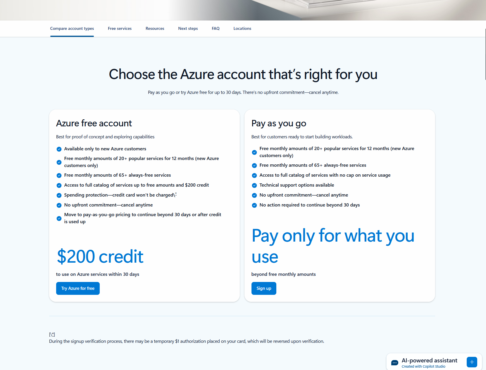
I first signed up for a Microsoft Azure free trial. A brand new Azure account is eligible for $200 of free credits to use within the first 30 days. This was perfect for learning and playing around with Azure as a beginner.
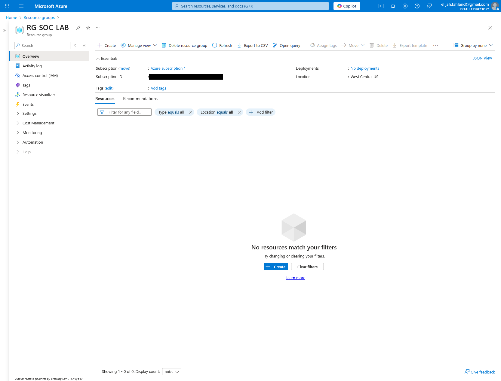
I then created a new resource group in Azure for the SOC lab. I aptly named it RG-SOC-LAB.
A resource group acts as a container for a bunch of related resources and allows for better organization and streamlined management in a variety of ways. It provides the ability to easily do things like monitor the associated Azure costs of a specific resource group (nice if I want to use this Azure account for other future labs), delete everything in the resource group with one easy swoop, and as I will come to do later, aggregate all the logs from the resources in this group into a single Log Analytics workspace. There are also other benefits to resource groups that aren’t within the scope of this lab.
Note that I’ve redacted my Azure subscription ID from this screenshot. Although a subscription ID isn’t highly sensitive on its own, exposing it could aid in social engineering attempts. Minimizing its visibility is a best practice for reducing unnecessary risk.
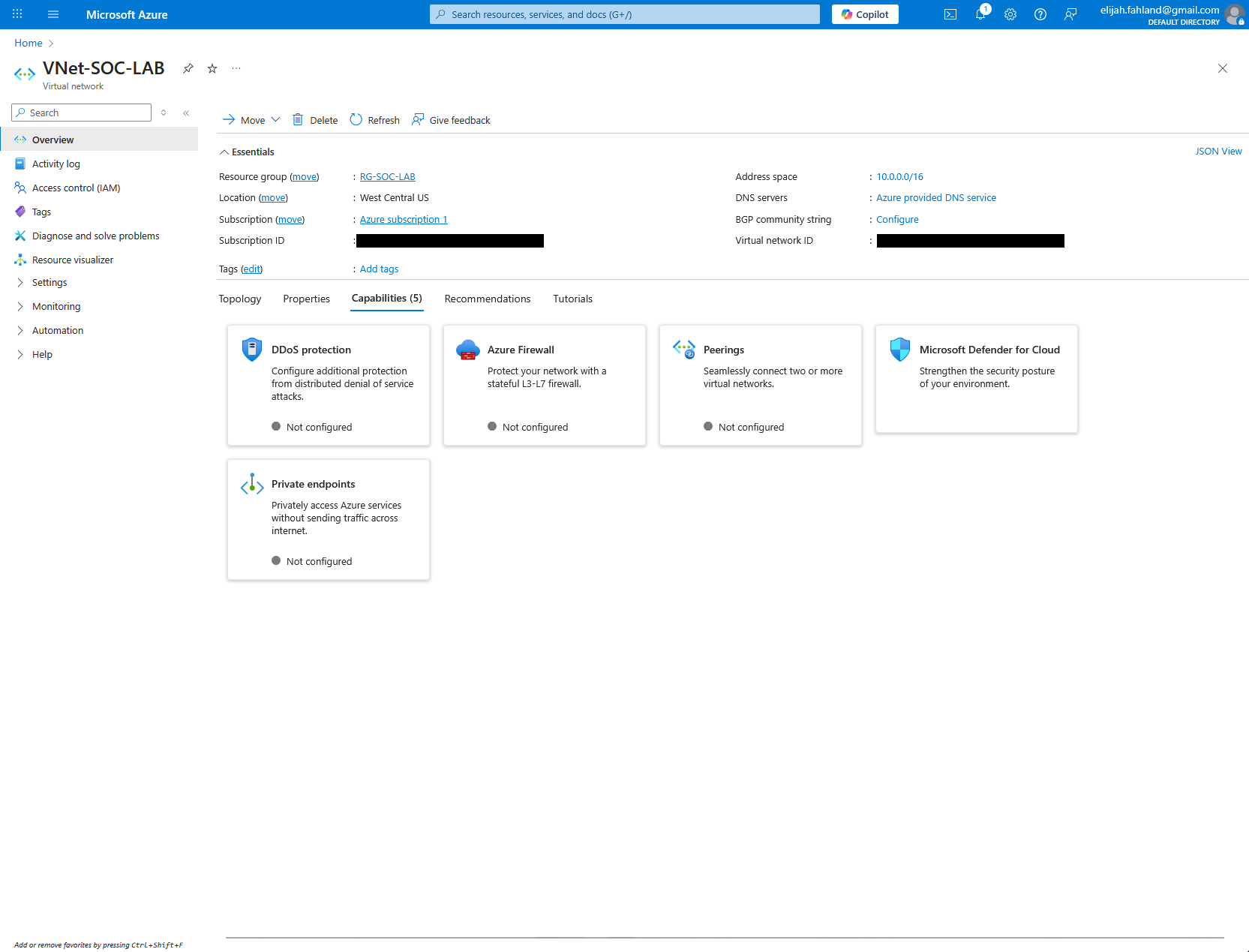
Next, I created a virtual network (also known as a VNet), which is Azure’s equivalent of a VPC on other cloud platforms, and placed it within the resource group I just created. All defaults were selected.
VNets provide a logically isolated network in Azure for cloud resources. While similar in concept to VLANs, which isolate traffic at Layer 2 in on-prem environments, VNets operate at Layer 3 and offer significantly more flexibility and control over IP addressing, routing, and security.
The next step was to create a virtual machine. This will ultimately end up as the target machine for the attackers to poke and prod at.
I gave it what I thought would be an enticing host name, should an attacker view it, and selected Windows 10 for the operating system. I select the default ‘Standard B1s’ size for the computer because Azure offers 750 hours for free with this size and it should still be adequate for this use case, despite its measly 1 virtual CPU core and 1 GB of memory. I had to change the availability zone to zone 3 as the free option was not available in the default zone 1. All other defaults were left as is.

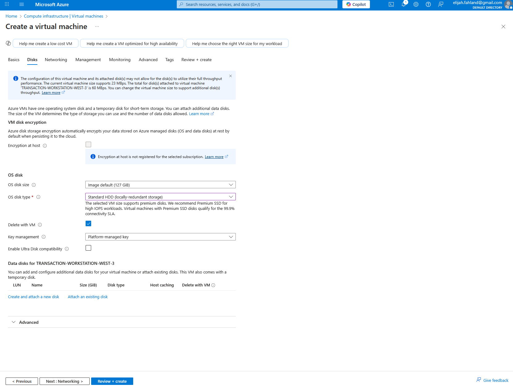
Since the VM size I selected has a maximum disk throughput of only 23 MBps, it wouldn’t be able to take advantage of the 100 MBps performance of the premium SSD option. For that reason, I opted for a standard HDD instead, which still provides up to 60 MBps, and is still more than the VM can utilize.
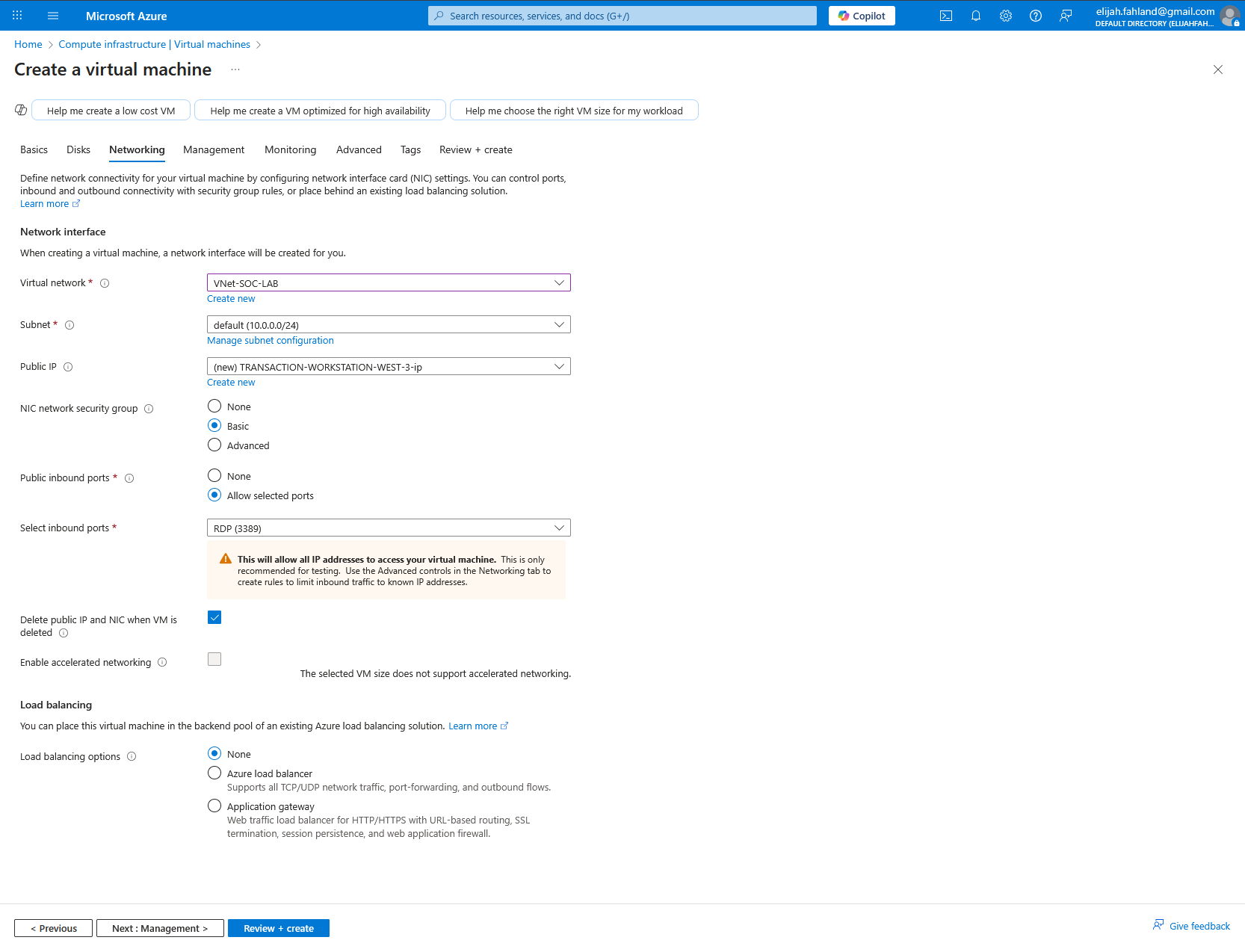
For the networking portion of the VM creation, the only default that was changed was checking the ‘Delete with VM’ checkbox which simply deletes the public IP addresses and NIC automatically, should I delete the VM. I ensured this VM was added to the VNet created earlier.
At this point I attempted to use Windows Remote Desktop Connection to login to the newly created virtual machine. This is where I quickly learned that the B1s VM size was absolutely not going to work for Windows 10! I had figured it would be slow as it only barely meets Windows 10 minimum requirements but it failed to make it past the ‘Out of the Box Experience’ setup wizard. Time to resize the VM!
This time I actually did a little research on what the minimum usable requirements for Windows 10 are, and while this is of course a little subjective, I settled on D2s_v3. Here is a quick comparison of how the B1s and D2s_v3 size specifications differ:

In addition to the differences in the specifications of each size, because these are from different families (B vs D), there are also differences in the subscription model of each.
The B family utilizes a bustable model that is best for workloads with primarily low CPU usage. It runs at a reduced CPU performance level but can burst up to the full rated CPU performance level when needed. This model uses something called CPU credits which act as a sort of currency or battery for this bursting. The VM consumes the CPU credits when bursting, and accrues the credits when at its reduced performance level. The CPU base performance level, maximum banked credits, CPU credit usage rate, and the accrual rate all vary depending on the specific B family VM size.
The D family utilizes a consistent performance model where full performance is always available.
In summary, D2s_v3 will offer much better performance for my Windows 10 machine and should have no issues receiving many attacks simultaneously.
To ensure I didn’t overuse my $200 credit, I made sure to be diligent about deallocating the virtual machine when I wasn’t actively using it.
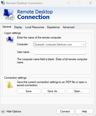
To connect to the Windows VM from my Windows computer I can utilize Window’s native Remote Desktop Connection program.
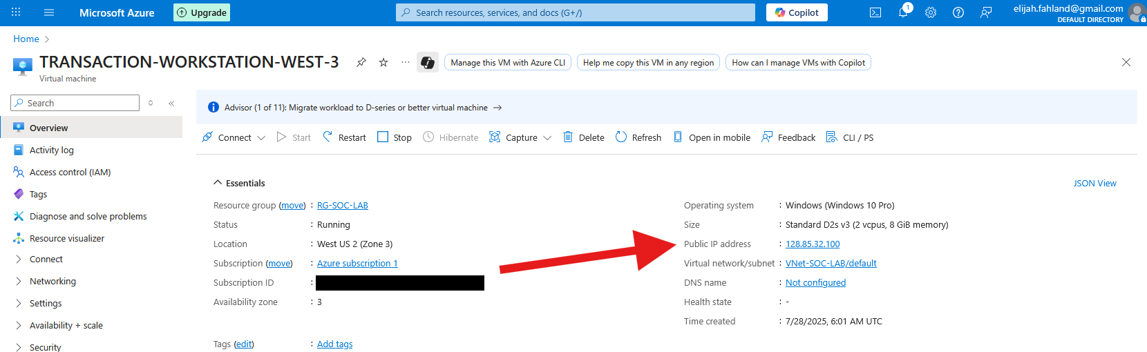
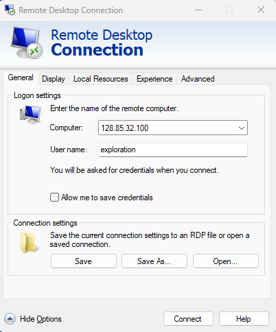
In the computer field I entered the public IP address of the VM. This can be found from within the VM Overview screen within Azure:
For the username, I just enter the one I made when setting up my VM. In this case, it’s: exploration.
It then be prompts for a password which is the same one I made when I set up the VM.
Note, at the time of this write up, this machine and all of it’s associated resources no longer exist.
Once logged in, the next step is going to be to make the target a little more delicious looking to attackers.
First I will open the firewall of the Network Security Group from within Azure. An NSG is a virtual firewall between the VM and the internet. In a home environment, it would be like the firewall on a home router.
Hopefully it goes without saying but this should never be done in an environment with anything of value.
Below are the default NSG rules.

Currently, the existing rules are set to only allow RDP connections. I’m going to delete this RDP allow rule and replace it with a rule that allows everything. Normally, this would be a terrible idea, but since I’m setting up a honeypot and there’s nothing of value on the machine, I’m okay with it. To clarify, I’m allowing any source IP address from any port to reach any destination address on any port.

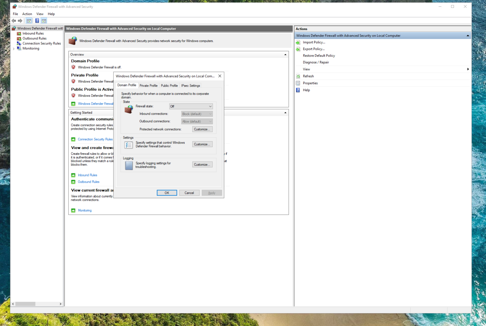
Next I will disable the Windows Defender Firewall entirely from within the VM.
Now that both the NSG and Windows Defender are opened up/disabled, I can check my work by pinging the VM’s IP address from my personal computer.
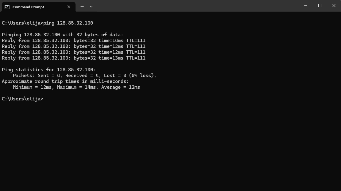
I am able to reach the machine from the internet so I know attackers can now do the same.
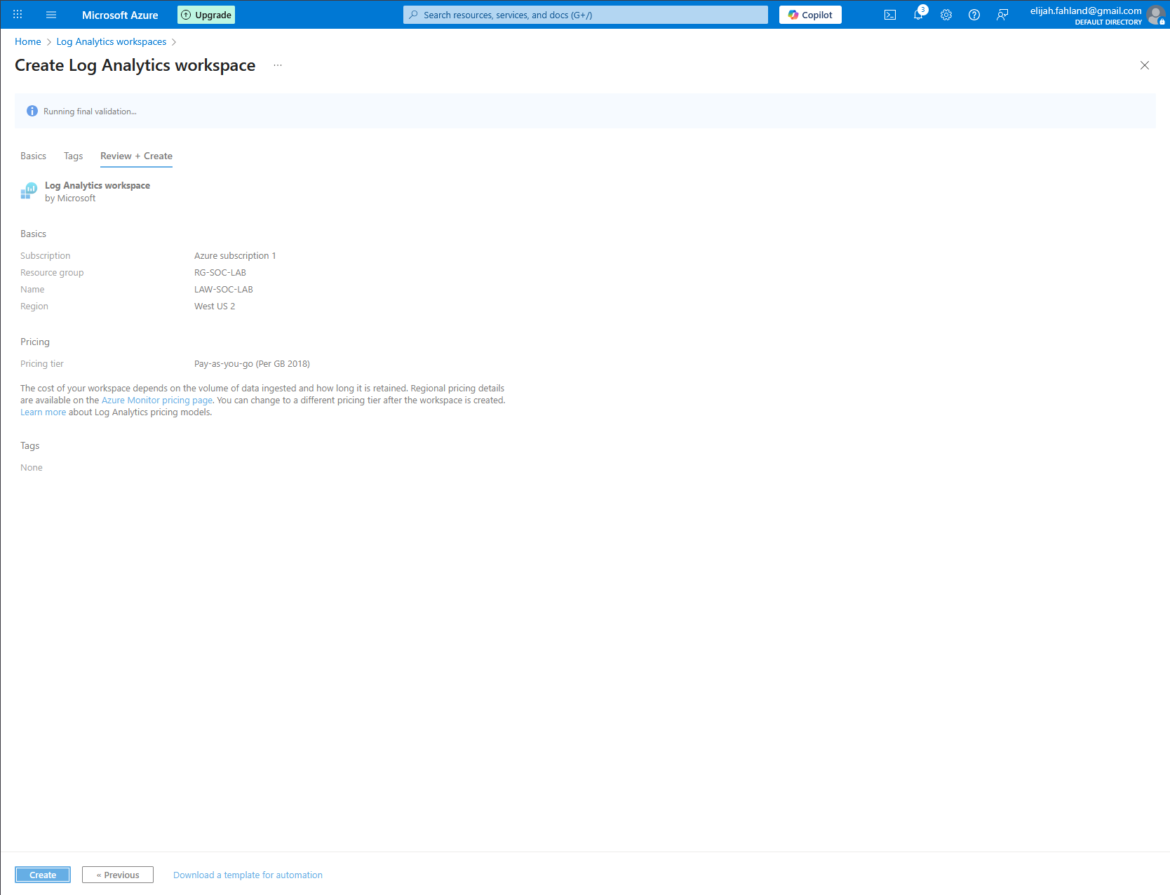
Next I will set up a new Log Analytics workspace within Azure. This is where all of the logs from our Windows VM will be aggregated so Microsoft Sentinel can access them. Microsoft Sentinel is cloud based SIEM which is able to collect, analyze, and respond to security events across many sources, all in one application.
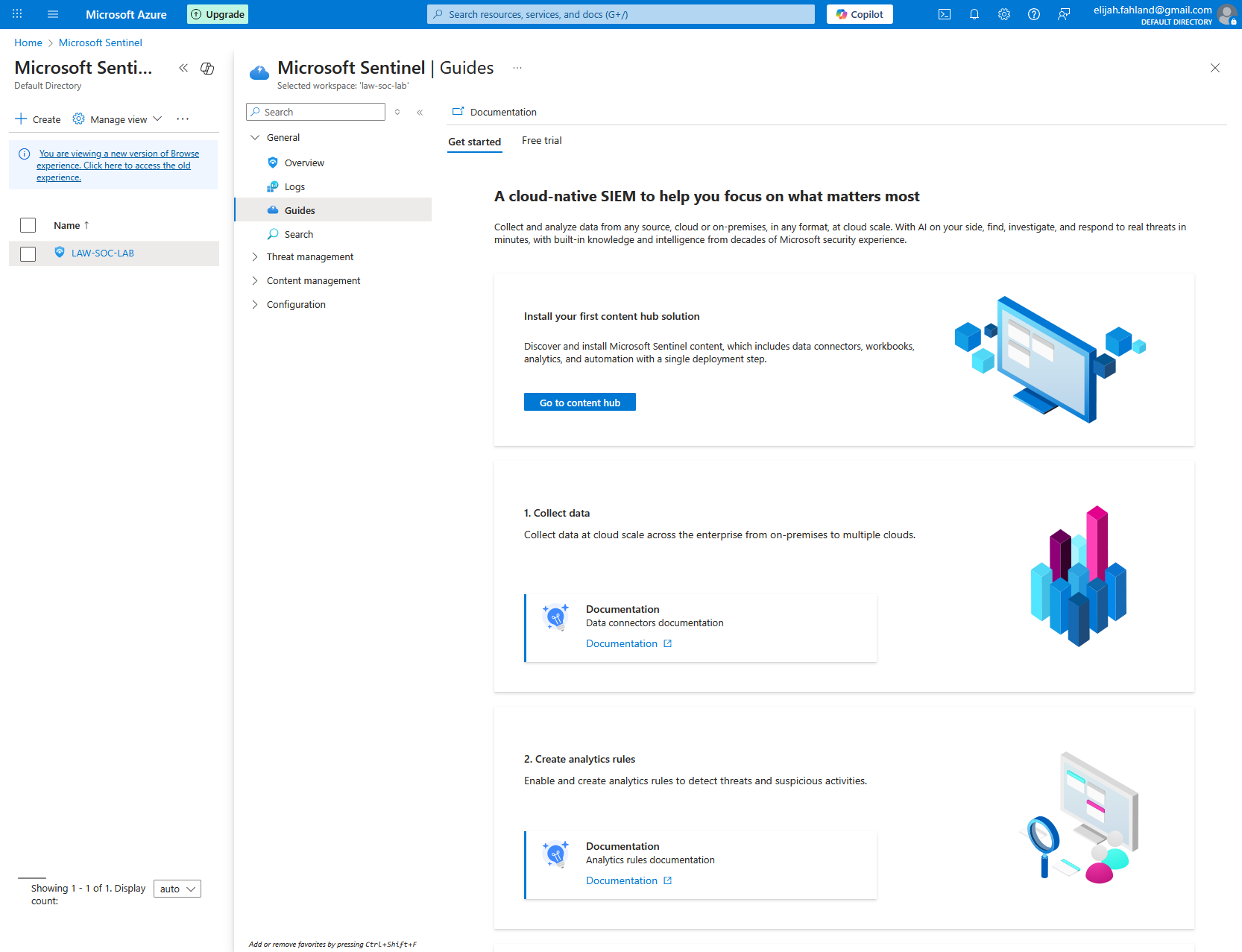
Next I set up Microsoft Sentinel with our newly created Log Analytics workspace. There are very few settings available during set up so here is the overview page once created.
Now I need to set up the VM to feed its logs into the Log Analytics workspace. I start by installing the Windows Security Events data connector onto our instance of Microsoft Sentinel.
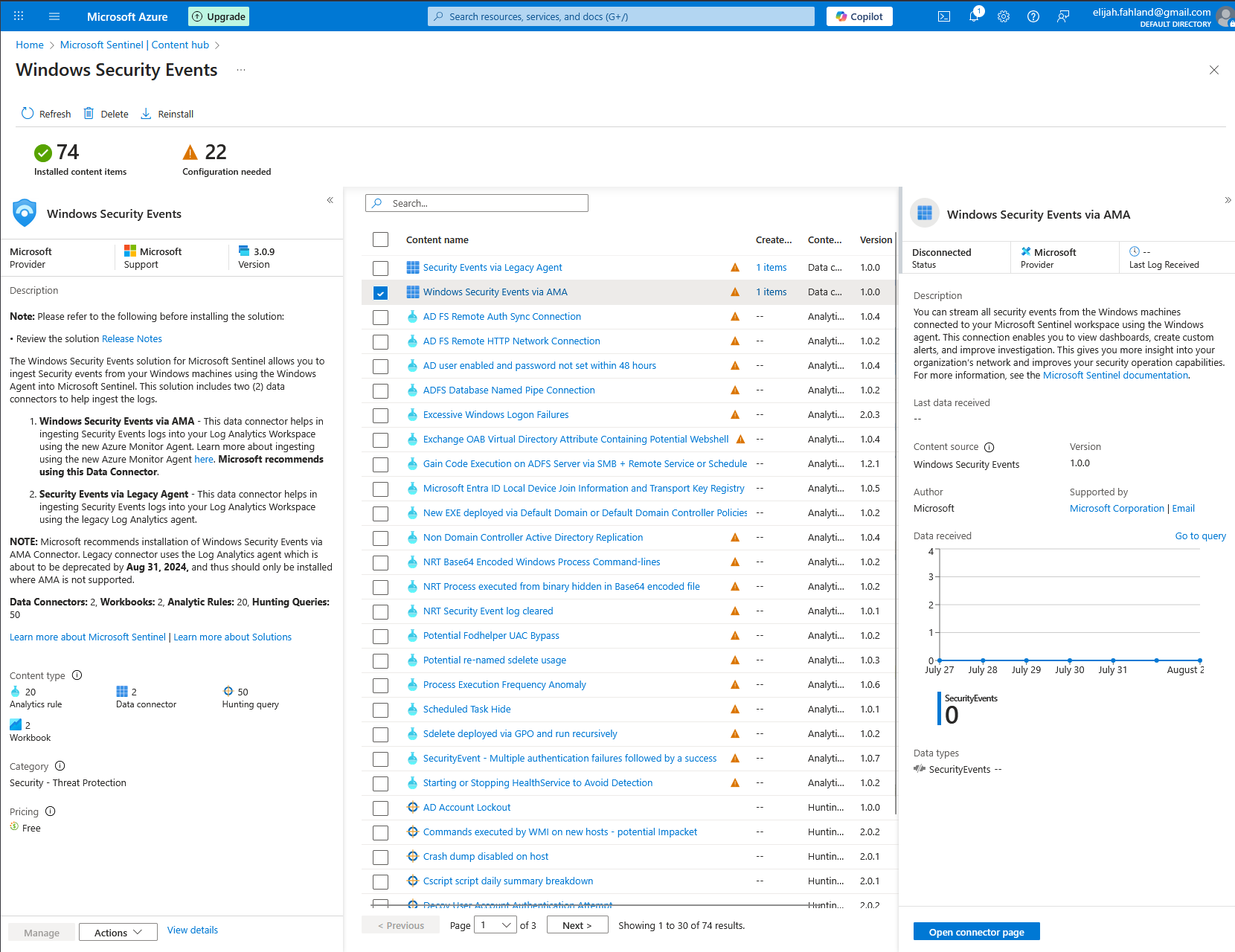
Here I select Windows Security Events via AMA and click on the open connector page button.
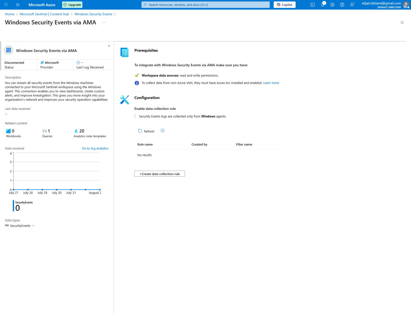
Next I will create a data collection rule. This rule is what tells the VM to forward logs into the Log Analytics workspace.
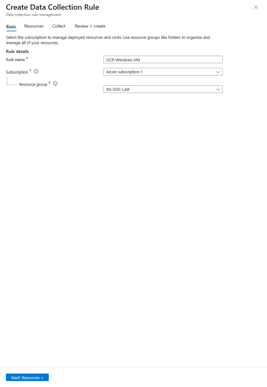
Here I give it a name and add it to the resource group I have been using.
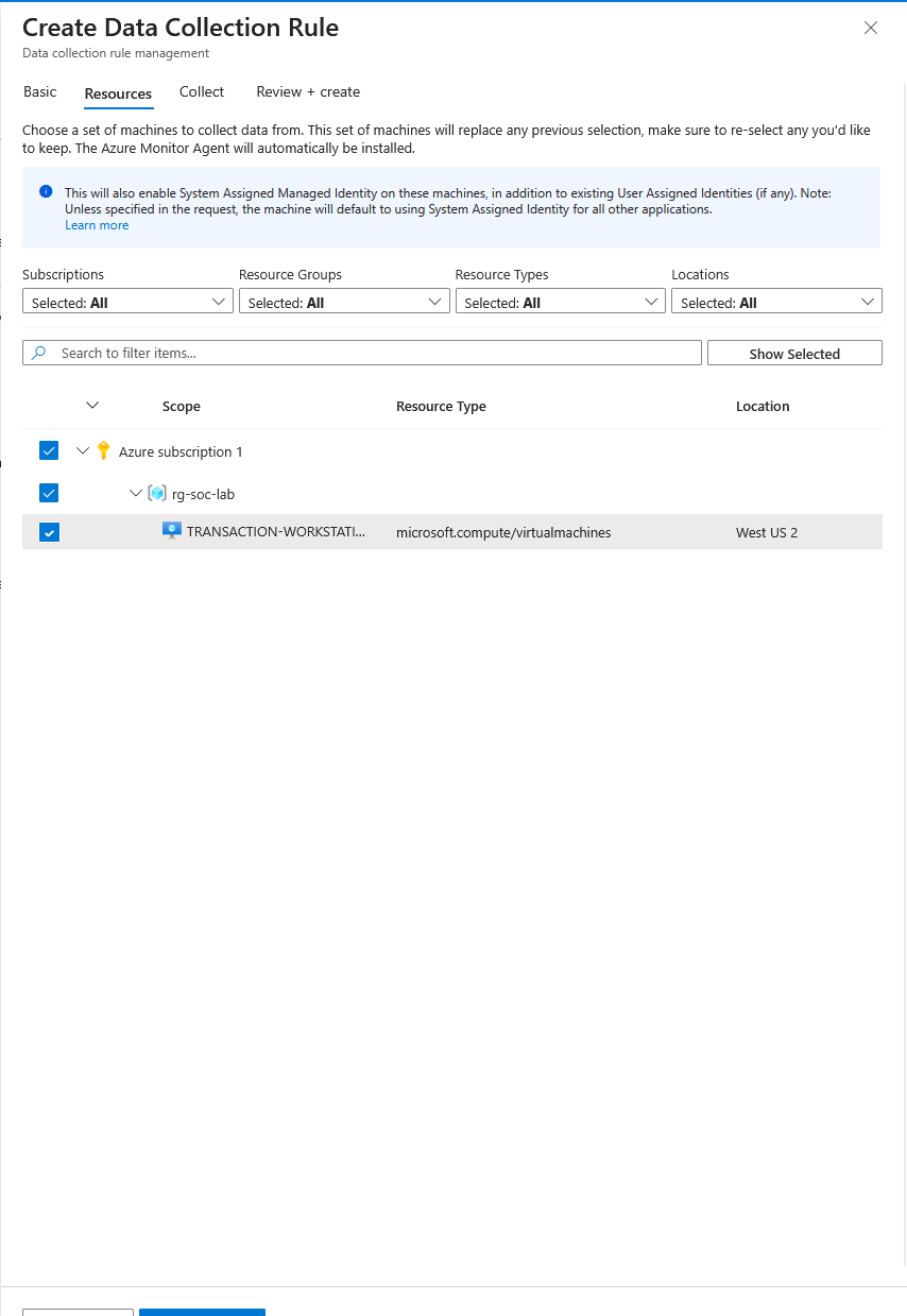
On this page I just select the virtual machine.
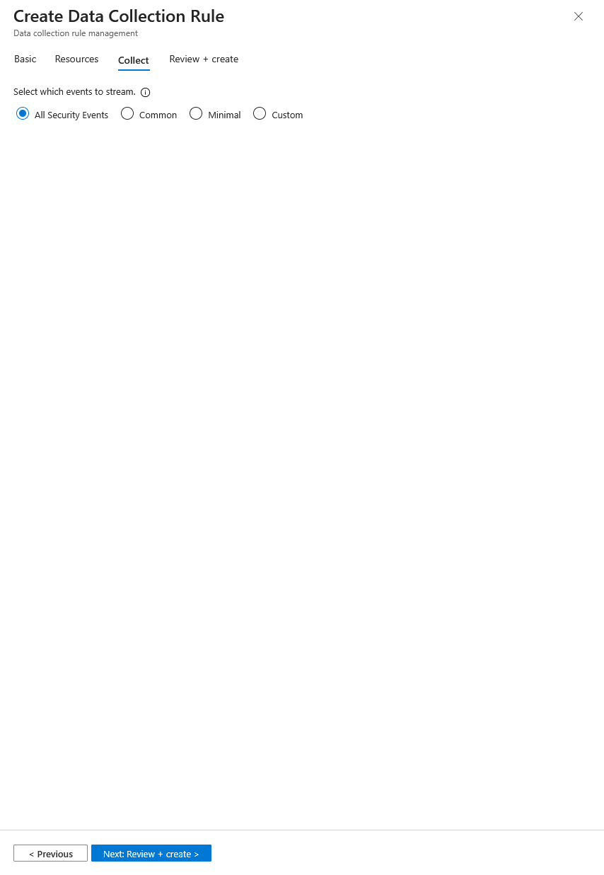
And finally I just select all security events before then selecting create.
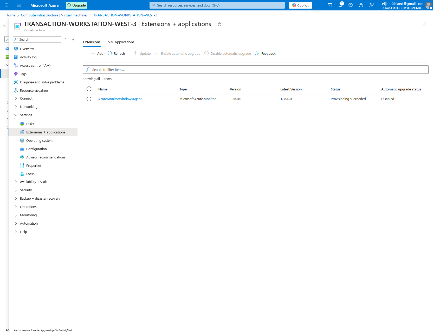
After that has all finished generating, I can navigate to the virtual machine and select extensions + applications. Here I see the AzureMonitorWindowsAgent being installed onto the virtual machine.
Now comes the exciting part. After waiting some time for the virtual machine to be discovered and prodded by attackers (not long at all), I can navigate back to our Log Analytics workspace and check to see if there are any logs available for viewing.
From within the Log Analytics workspace I have the ability to query the logs using KQL (Kusto Query Language). KQL is a query language somewhat similar to SQL except it's specifically designed for querying logs instead of relational databases, and is also fittingly read only.
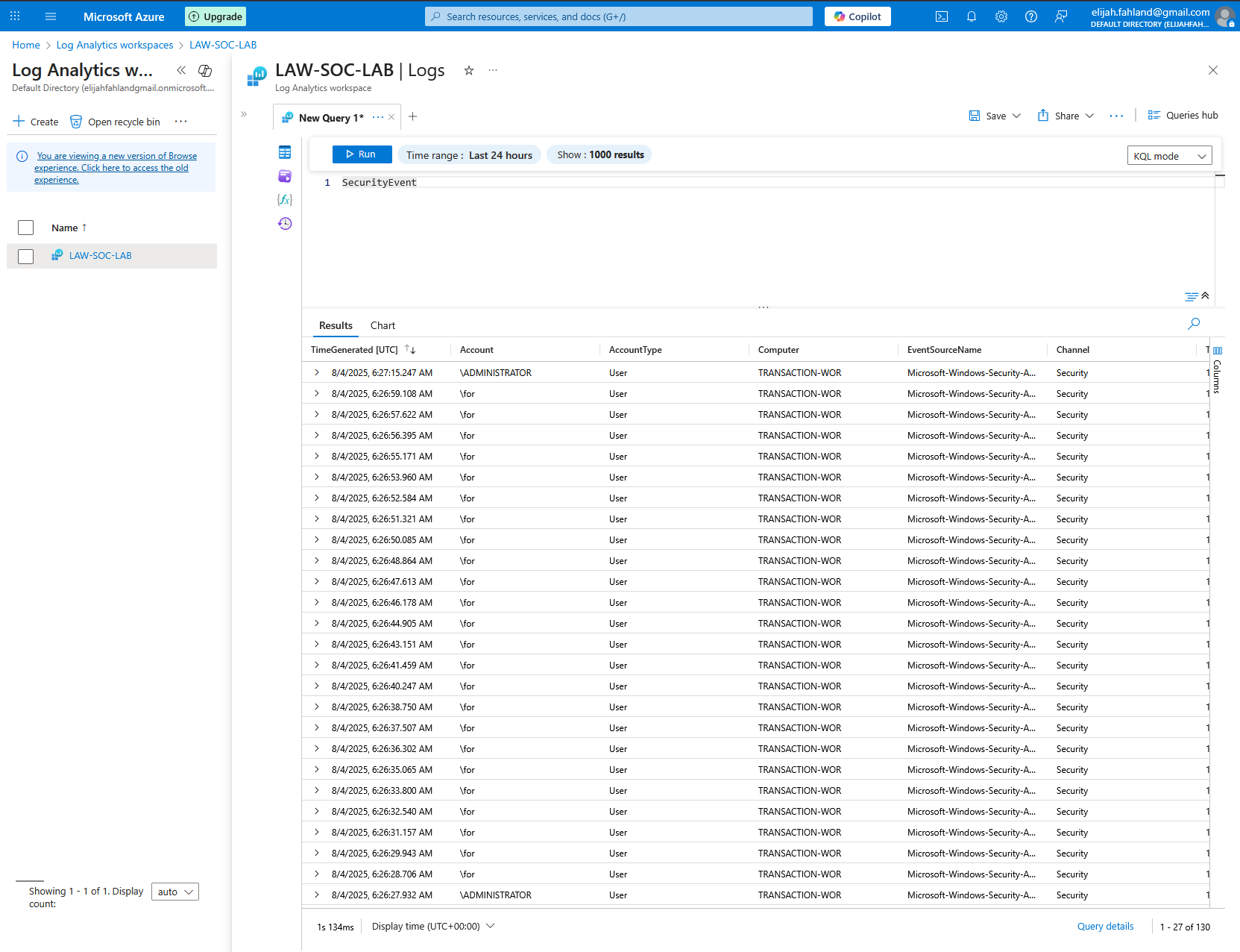
Entering ‘SecurityEvent’ as a query returns all logs from the SecurityEvent table. This is the table associated with things such as logon attempts, audit events, and privilege use.
As can be seen from the results of the query, the Windows VM is already being attacked.
I can also refine the query to only show certain types of events. For example, I am most interested in seeing failed logon attempts which is EventID 4625. I can use the query below to restrict the results to failed logon attempts and also order them from newest to oldest.
SecurityEvent
| where EventID == 4625
| sort by TimeGenerated desc
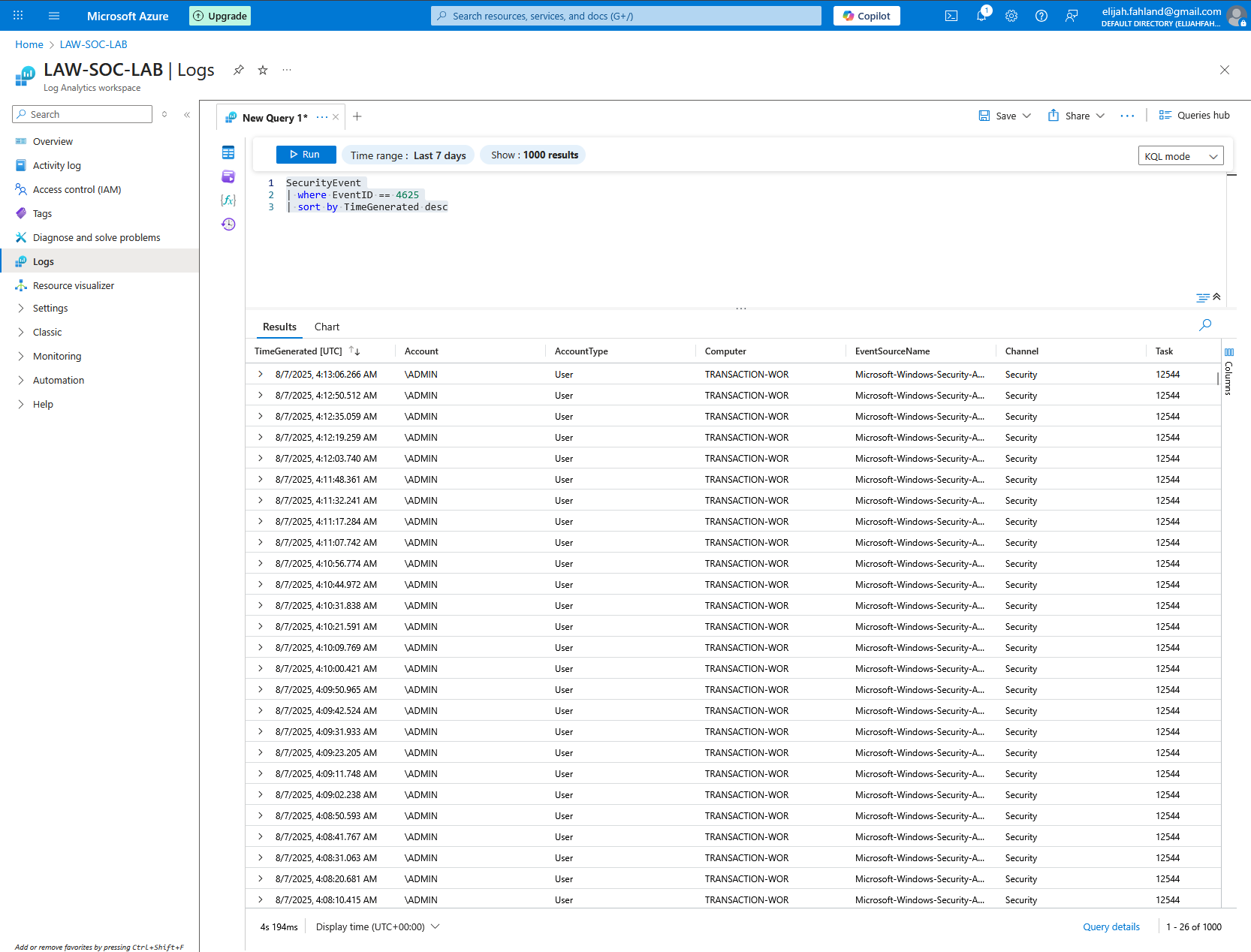
It looks like there are already have a ton of logs!
For the next stage I am going to plot the supposed geographic locations of the attackers from each failed logon onto a map so I can see where in the world the VM is being targeted from. Each log contains a source IP address but of course there isn’t any geographic data (such as a city, country, or latitude and longitude). I will need a way to associate the IP addresses to a physical location.
One quick point worth mentioning is that IP addresses are not a particularly reliable indicator of someone’s true location. IP based geolocation is based on public registry and network routing data, which can be outdated, imprecise, or intentionally obscured. Factors like the use of VPNs, proxies, cloud hosting providers, and mobile networks can make an IP appear to originate from a completely different region than the actual user. Despite this, it will still be really neat to see the IP addresses plotted on a map.
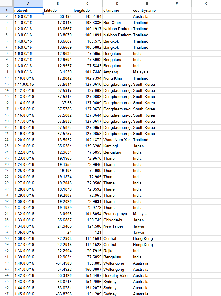
To do this I will first need additional data which associates IP addresses with geographic locations. I have a beautiful CSV (Credit to Josh Madakor for providing this CSV) with blocks of IPs and their general geographic locations in the form of latitude and longitude, city, and country. Below is a screenshot of what some of the data looks like.
Next I add a Watchlist to Microsoft Sentinel. A watchlist is basically just a custom table which I can use to query with the logs in the Logs Analytics workspace using KQL. An example of a common use case would be a watchlist which contains a list of known malicious IP addresses which you could then use to compare against incoming traffic logs in order to identify potential bad actors.
Below is what the file looks like after it’s been fully uploaded.
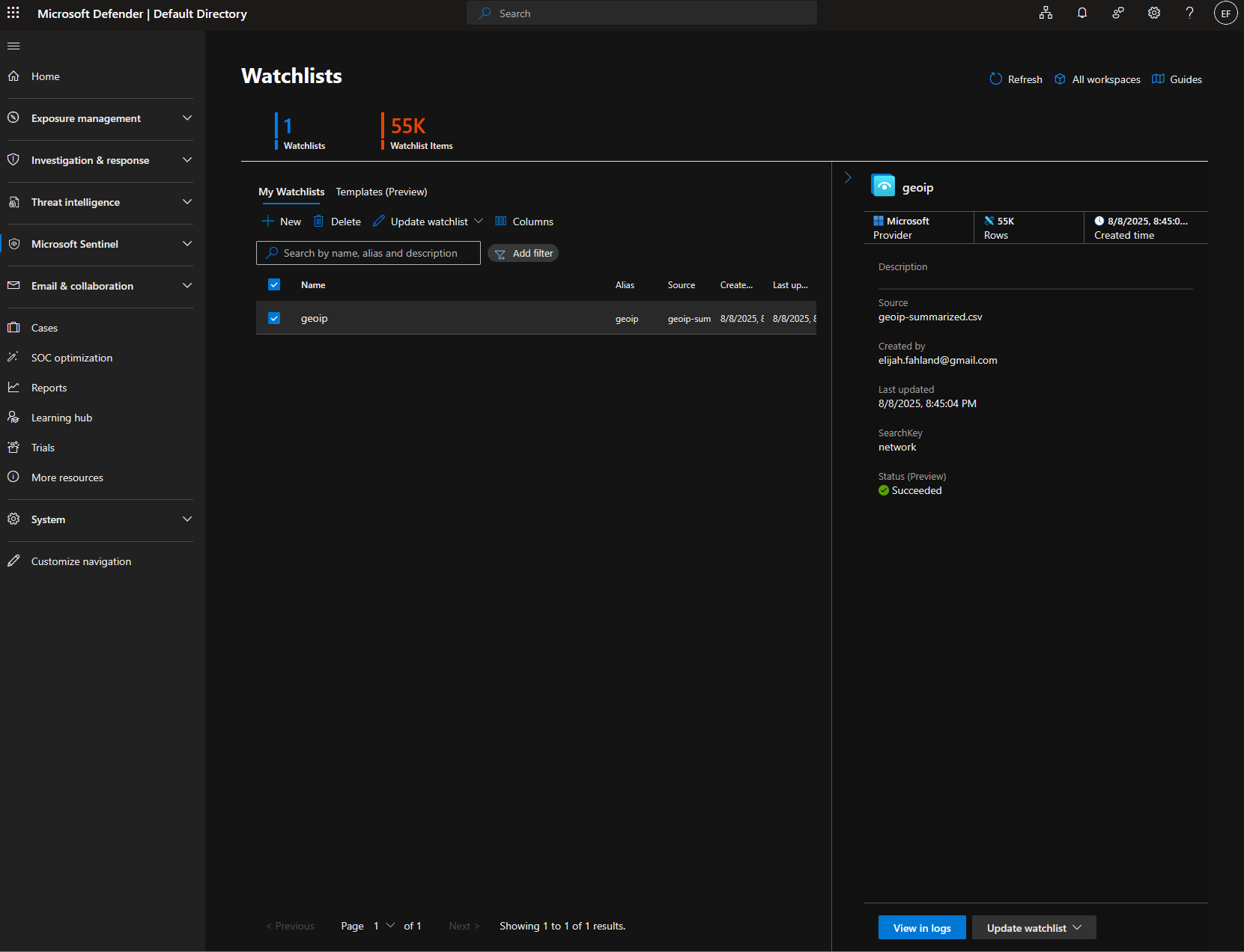
You can see there are now 55,000 watchlist items which aligns with the approximately 55,000 thousand rows from the CSV file.
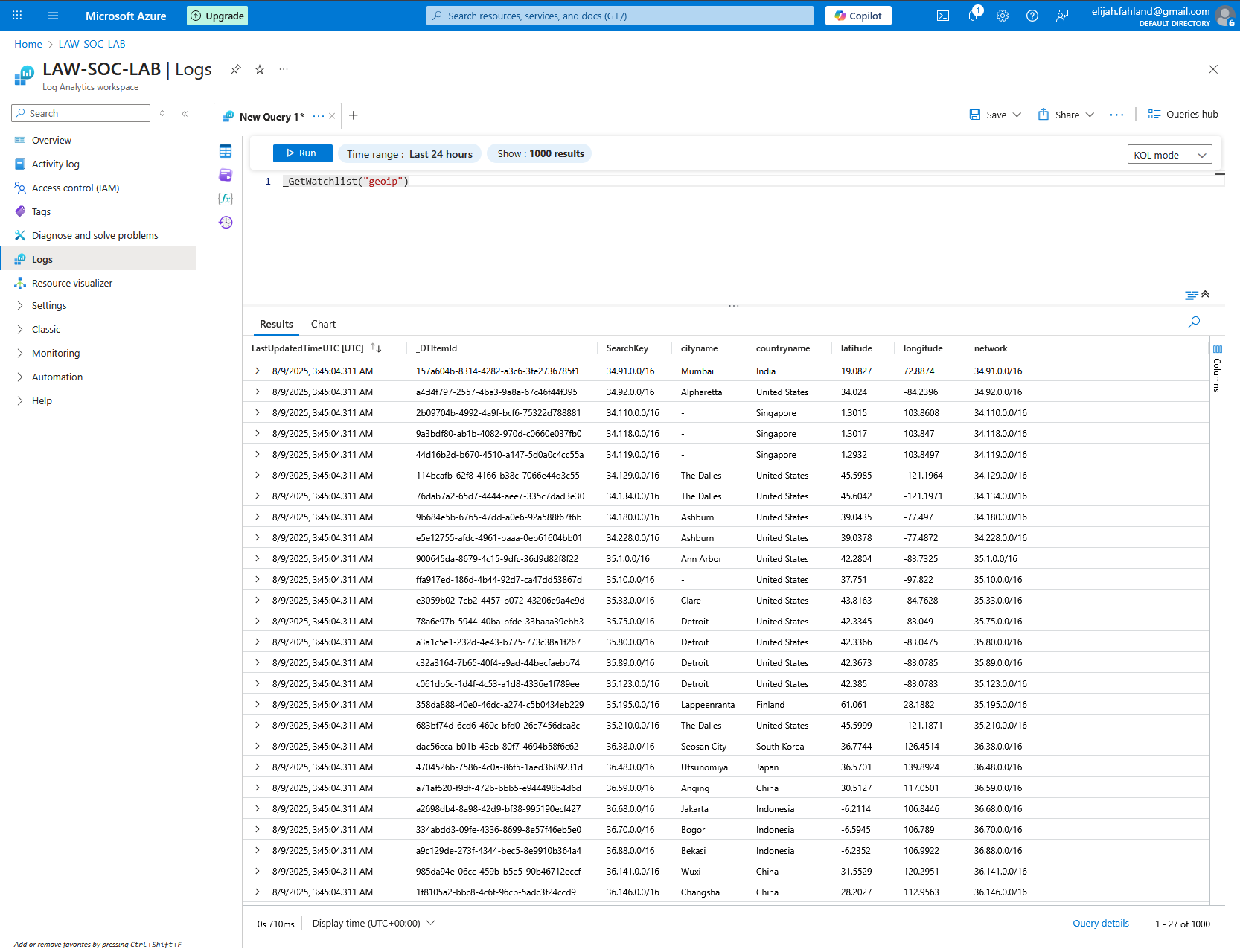
Now we can go back and ensure everything is working correctly by querying our watchlist from within our Log Analytics workspace. We will use the following command within KQL:
_GetWatchlist(“geoip”)
The results of this query show all columns and the first 1000 rows of our CSV.
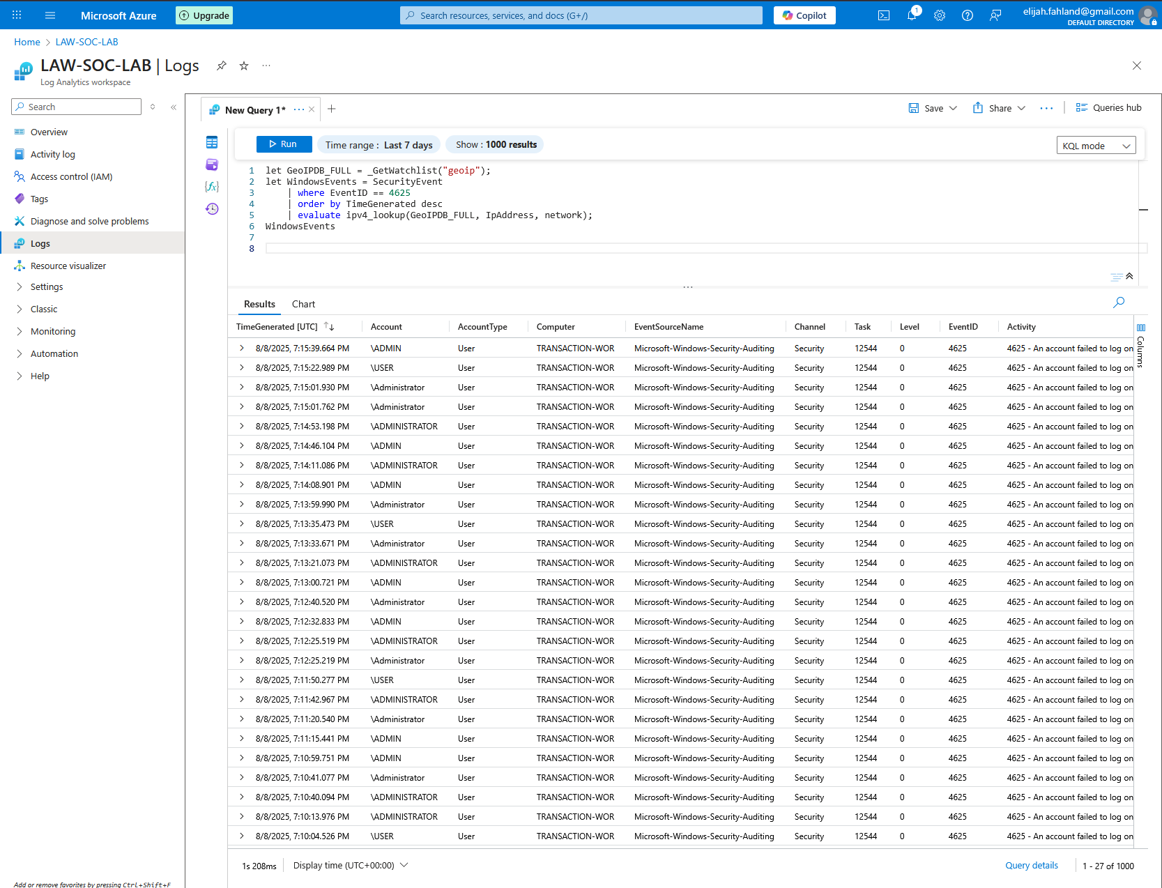
The following query below will enrich our existing logs by joining the new location data, so I can see the geographic location of each failed login attempt.
1 let GeoIPDB_FULL = _GetWatchlist("geoip");
2 let WindowsEvents = SecurityEvent
3 | where EventID == 4625
4 | order by TimeGenerated desc
5 | evaluate ipv4_lookup(GeoIPDB_FULL, IpAddress, network);
6 WindowsEvents
I will break down what each line does:
Creates a variable called GeoIPDB_FULL and assigns the geoip watchlist to it which can be referenced later
Creates another variable called WindowsEvents and assigns the SecurityEvent table to it (which contains all of the Windows security event logs from the VM), in accordance with the additional queries from lines 3-5
Restricts the results to only those with an EventID is 4625 (a failed logon)
Orders the results by the TimeGenerated column in descending order (most recent dates at the top)
Uses the evaluate operator to run the ipv4_lookup function, which matches the IP address from the VM’s logs to the corresponding IP range in the geoip watchlist
Returns the newly created and enriched table just made
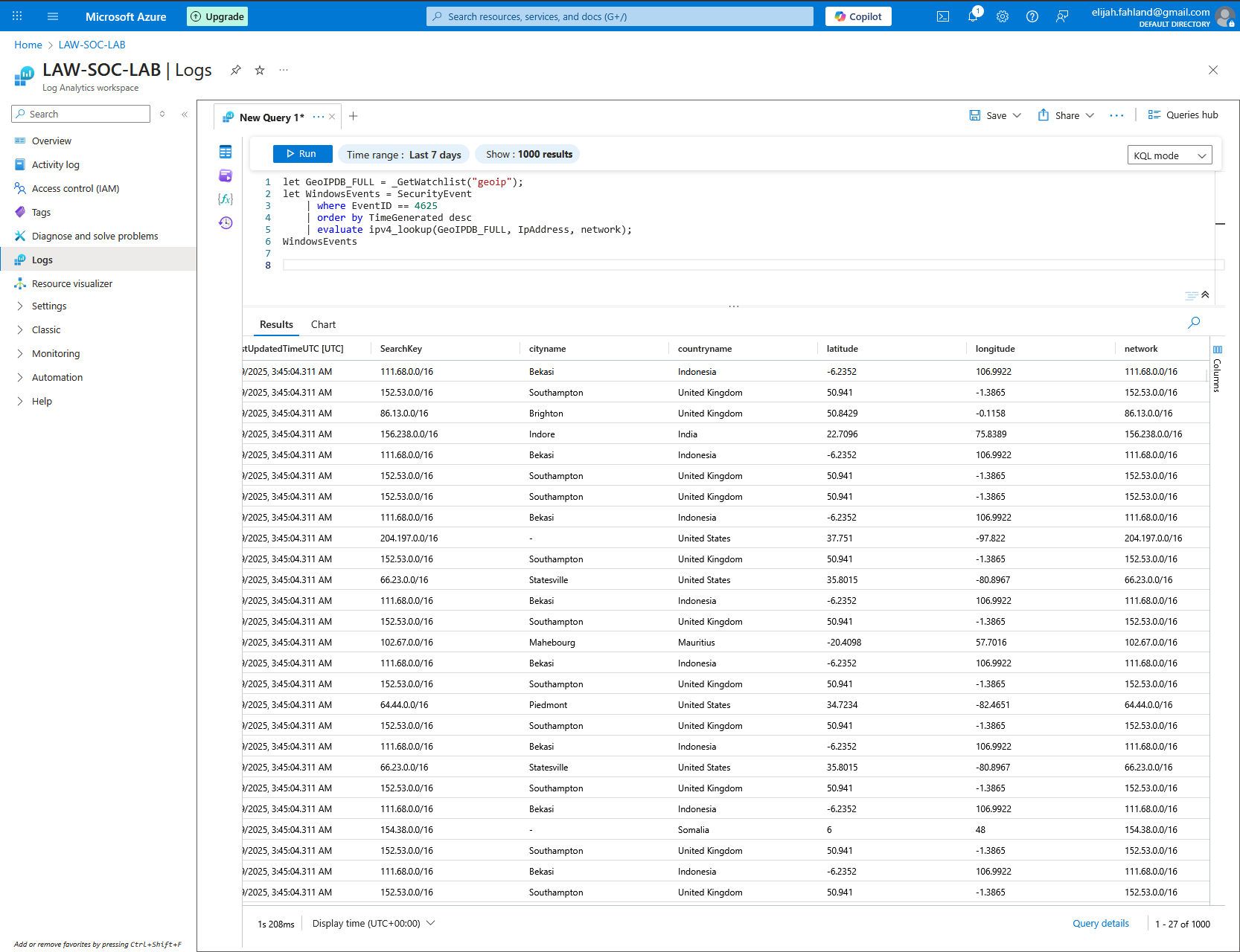
Below are the results of this query. It has a lot more data per row now.
The geographic locations are all the way to the right as you can see below.
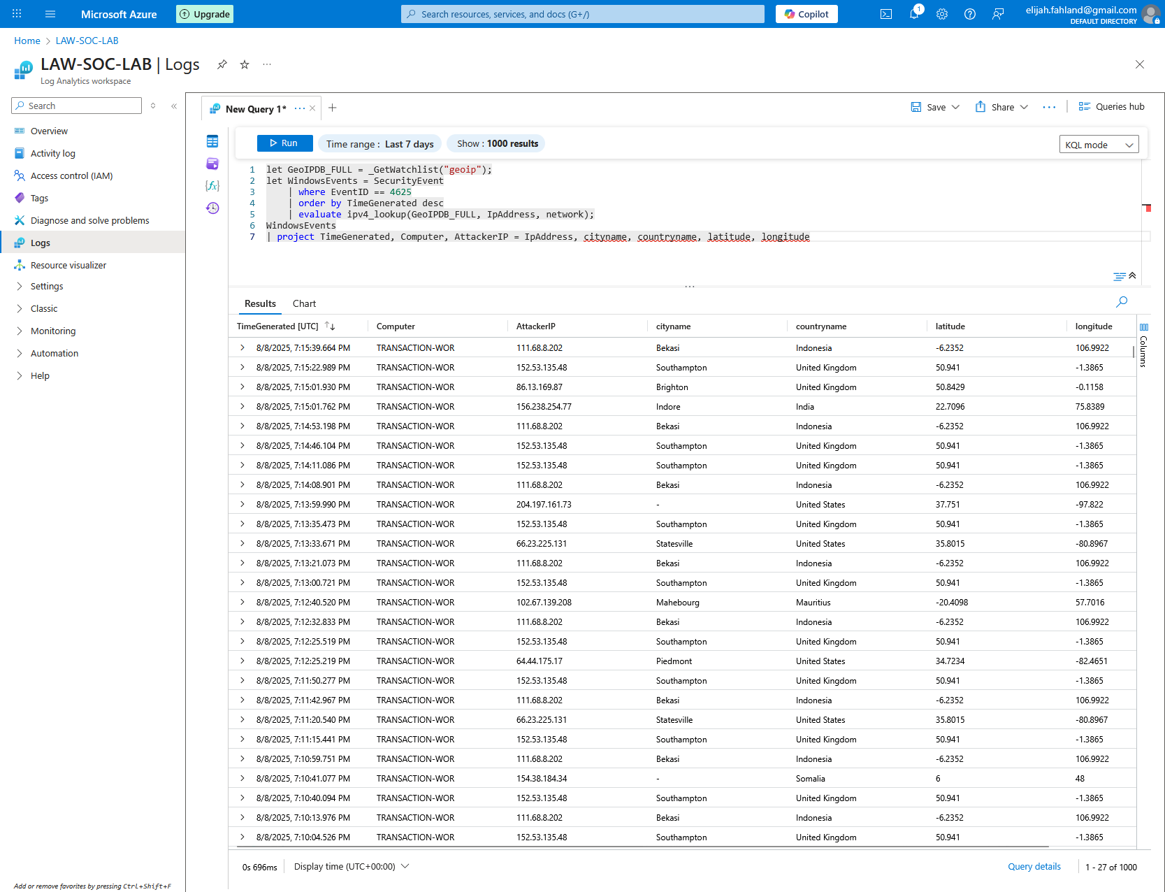
I can clean up the results by using the project operator to restrict the returned columns and renaming one of them for clarity:
let GeoIPDB_FULL = _GetWatchlist("geoip");
let WindowsEvents = SecurityEvent
| where EventID == 4625
| order by TimeGenerated desc
| evaluate ipv4_lookup(GeoIPDB_FULL, IpAddress, network);
WindowsEvents
| project TimeGenerated, Computer, AttackerIP = IpAddress, cityname, countryname, latitude, longitude
The revised query returns this:
The final step will be to map these on an actual map to make the data easier and faster to understand. I will start by adding a new workbook within Sentinel.
From this screen I will select edit and delete the two default queries so there will be a blank slate. Then I will add a new query, select the advanced editor, and paste in a snippet of JSON (Credit to Josh Madakor for providing this JSON).
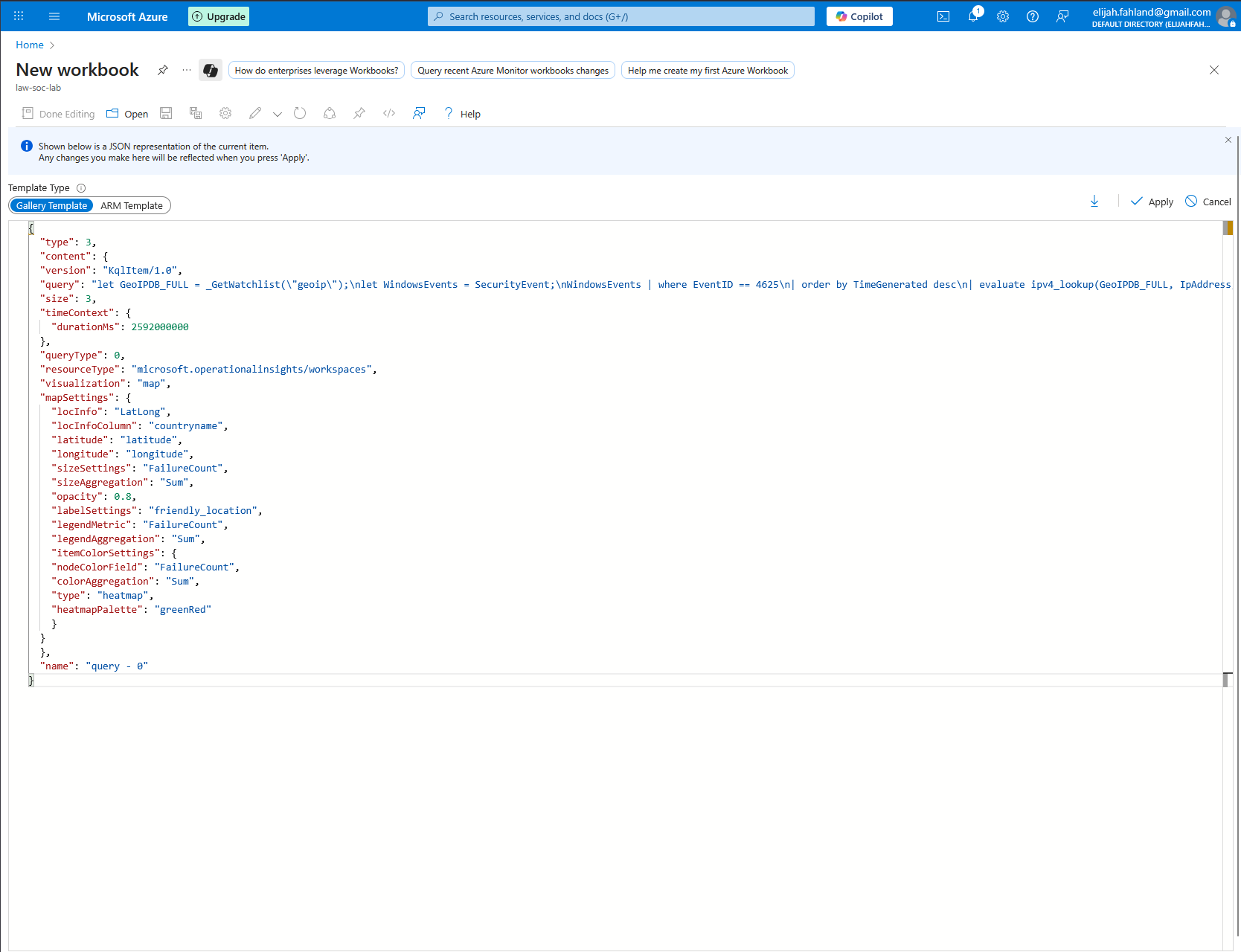
Let me walk through some of the more interesting lines and discuss what is happening in this code:

Lines 2-4 tell Azure Workbooks this element is a KQL query visual. This just tells Workbooks how to interpret and display the item.
Lines 5-12 is a KQL query which is very similar to the last one I created. Here is a quick reminder and rundown of what it does:
Assigns the geoip watchlist to the GeoIPDB_FULL variable
Assigns the filtered SecurityEvent table to the WindowsEvents variable (see SecurityEvent filters below)
Filters to only show failed logons (where EventID is 4625)
Orders newest first (not technically necessary here)
Uses the evaluate operator to run the ipv4_lookup function, which matches the IP address from the VM’s logs to the corresponding IP range in the geoip watchlist
Counts up all rows which contain the same IP address, latitude, longitude, city name, and country name and assigns the number to the variable FailureCount
Returns relevant columns and renames some of them for clarity; uses strcat to concatenate city and country into one easy to read header
Line 13 simply sets the size of the tile within the workbook.
Line 14 and 15 set the query data range to the last 30 days in milliseconds
Line 17 sets the query type as 0, which is a standard KQL query
Line 18 tells the workbook that this query should run against the Log Analytics workspaces
Line 19 simply tells the workbook to render the query results on a map instead of a table
Lines 20-35 are the settings for the map. For the most part they are fairly intuitive to understand. A few key points to make are that we use the latitude and longitude data for plotting on the map, FailureCount as the primary metric and for sizing/coloring the plots, and friendly_location (city and country) as the text labels for each plot and the legend.
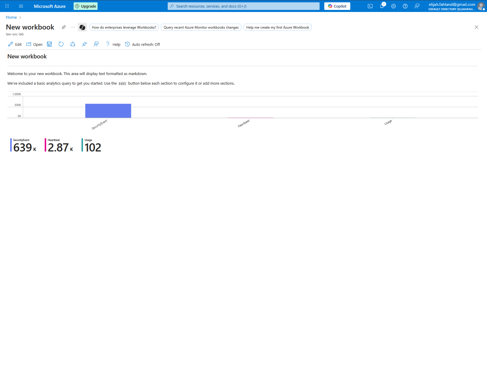
After adding the JSON, I will save and place it into our existing resource group. Now the new map with the attackers' geographic locations plotted on it is visible:
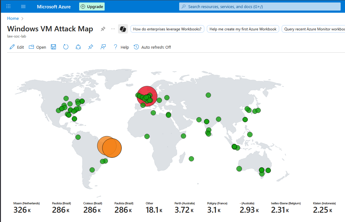
The numbers at the bottom represent the number of attacks from those locations over the last 30 days. However the VM was only turned on for a total of about 4 days!
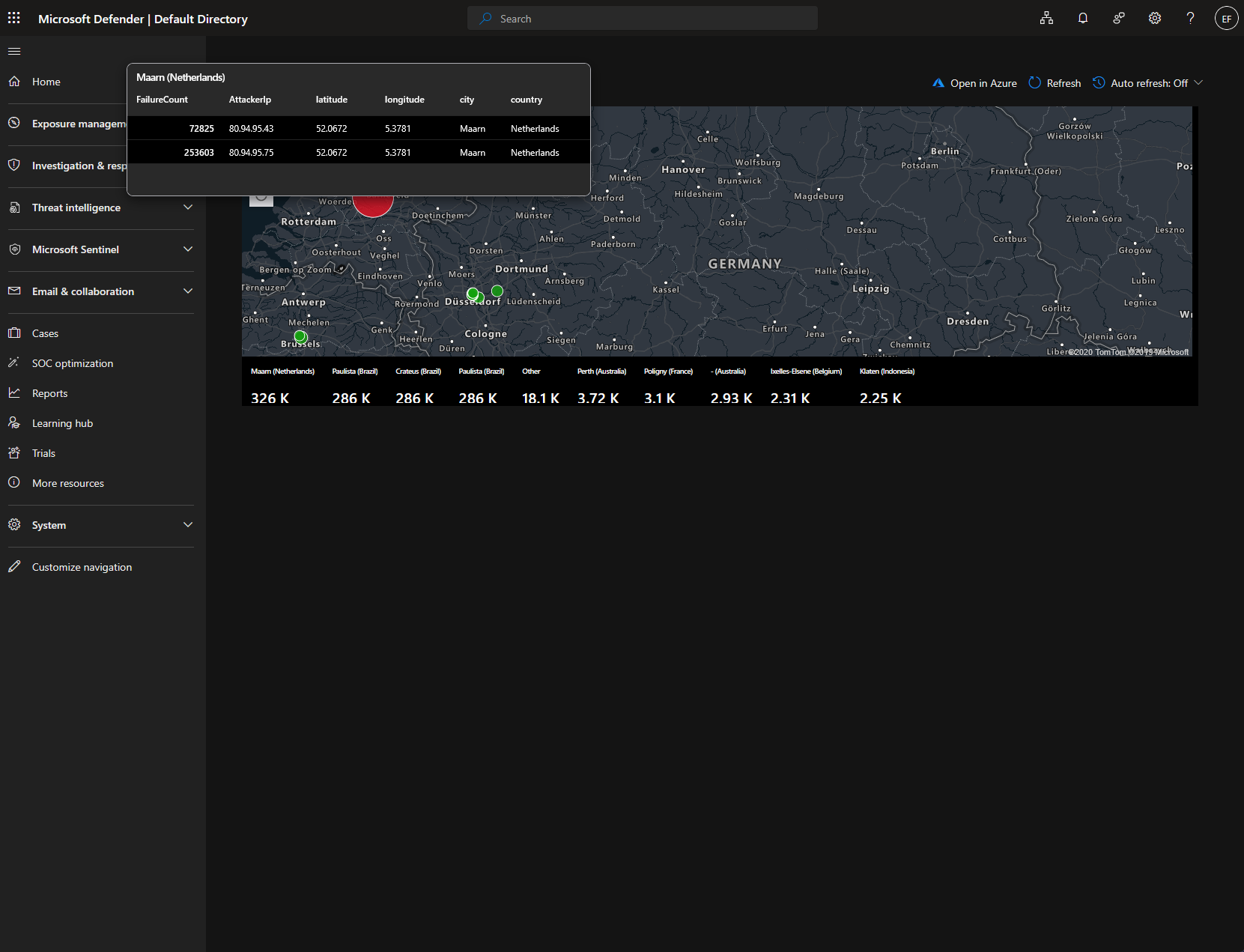
If I access the workbook from within the Microsoft Defender interface I can also interact with the map a bit more. I can scroll and zoom around our map and click on the various plots to view more information, such as the attacker IP address and number of attacks.
As is, there is a fair bit of really interesting information to enjoy from the logs. It’s obviously quite neat getting to see where the majority of attacks originated from and how quickly they are made. At this point however I haven’t done anything but gather information!
Some obvious next steps I will be circling back around to in the near future will include:
Adding automation to control the attacks, for example, automatically blacklisting IP addresses after a specified number of failed logon attempts
Building custom detection rules, such as writing Sentinel queries to trigger alerts on suspicious patterns like password spraying, brute force attempts, or certain geographic locations
Correlate with threat intelligence: Compare attacker IPs against data from AlienVault OTX for example
I hope you have enjoyed this write up as much as I did making it!